Data Imputation Techniques: Handling Missing Data in Machine Learning

Handling missing data is one of the most common challenges in machine learning. Real-world datasets are often incomplete, which can impact model performance and the reliability of analysis. Whether it’s due to sensor errors, user input mistakes, or data collection issues, missing data must be addressed carefully. Data imputation is the process of filling in missing data points to ensure that the dataset is complete and ready for analysis. In this blog, we’ll explore some common and advanced data imputation techniques like mean, median, mode imputation, K-Nearest Neighbors (KNN) imputation, and Multiple Imputation by Chained Equations (MICE).

The Importance of Data Imputation

Missing data can skew results, reduce the predictive power of models, and lead to biased conclusions. Machine learning algorithms like decision trees or linear regression require complete datasets to function optimally. In some cases, simply ignoring or deleting rows with missing values can lead to a significant loss of data and crucial insights. Imputation helps retain most of the dataset’s useful information by replacing missing values with plausible estimates.

Types of Missing Data

Before diving into imputation techniques, it’s important to understand the types of missing data:

1. Missing Completely at Random (MCAR):
   Missing values occur entirely at random and have no relationship to any other variables in the dataset.
2. Missing at Random (MAR):
   Missing values are related to other observed variables but not the missing variable itself.
3. Missing Not at Random (MNAR):
   Missing data is directly related to the value that is missing. For example, high-income individuals may not report their income in a survey.

Understanding the type of missing data can help you choose the most appropriate imputation method.

Common Imputation Methods

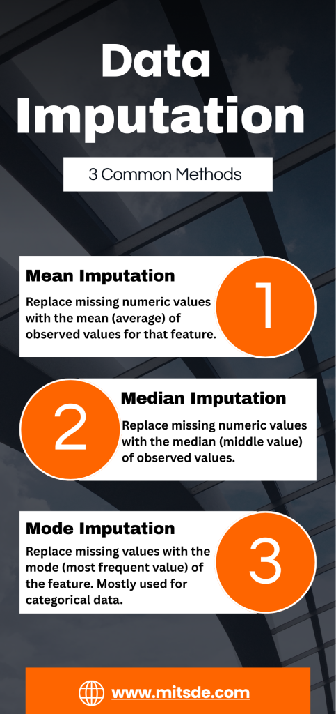
1. Mean Imputation

Mean imputation is a simple and widely used technique for handling missing data. It involves replacing missing values with the mean (average) of the observed values for that particular feature.

Example: If the feature Age has missing values, you calculate the mean age from the available data and replace missing values with this mean.

Pros:

• Simple and quick to implement.
• Works well when the data is MCAR and not skewed.

Cons:

• Can distort the distribution of the data, particularly if the data is skewed.
• Reduces variance, which can affect model performance.

2. Median Imputation

Median imputation is similar to mean imputation but uses the median instead of the mean. This is useful when the data is skewed, as the median is less affected by outliers than the mean.

Example: For a feature like Income, which may be skewed by a few very high values, median imputation can be more appropriate.

Pros:

• More robust to outliers than mean imputation.
• Preserves the data’s central tendency better in skewed distributions.

Cons:

• Like mean imputation, it ignores relationships between variables, which can lead to inaccurate imputation.

3. Mode Imputation

Mode imputation replaces missing values with the most frequent value (mode) of the feature. This technique is particularly useful for categorical data.

Example: For a categorical feature like Gender, you can impute missing values with the most frequent category, such as “Male” or “Female.”

Pros:

• Simple and effective for categorical variables.
• Preserves the distribution of categories.

Cons:

• May introduce bias if the most frequent category is overrepresented.

Advanced Imputation Techniques

1. K-Nearest Neighbors (KNN) Imputation

K-Nearest Neighbors (KNN) imputation is a more sophisticated method that looks at the “k” closest data points (neighbors) to estimate the missing values. It works by finding the k-nearest points based on the distance (usually Euclidean distance) from the point with missing data. The missing value is then imputed based on the average (for numerical data) or the mode (for categorical data) of these neighbors.

Example: For a missing value in the Age feature, KNN finds the k nearest records based on other features like Income or Occupation and imputes the average age of those neighbors.

Pros:

• Takes into account the relationships between multiple variables, making it more accurate.
• Works well for both numerical and categorical data.

Cons:

• Computationally expensive, especially with large datasets.
• Sensitive to the choice of k and the distance metric.

2. Multiple Imputation by Chained Equations (MICE)

MICE is an advanced method that iteratively imputes missing values by modeling each feature as a function of other features. It creates multiple imputed datasets, fits a model to each one, and then pools the results for a final imputation.

The process works as follows:

1. Impute missing values with simple methods (mean, median, etc.) initially.
2. Select one feature and regress it on the other features with imputed values.
3. Use the regression model to predict missing values for that feature.
4. Repeat this process for all features multiple times.

Pros:

• One of the most accurate methods because it takes into account relationships between variables.
• Handles both numerical and categorical data.
• Can provide multiple imputations, which can be averaged for better estimates.

Cons:

• Computationally intensive and requires specialized software like R or Python’s statsmodels library.
• Requires careful tuning and understanding of the relationships between variables.

Best Practices for Choosing an Imputation Method

Choosing the right imputation method depends on the type of data, the amount of missing data, and the relationships between variables. Here are some guidelines:

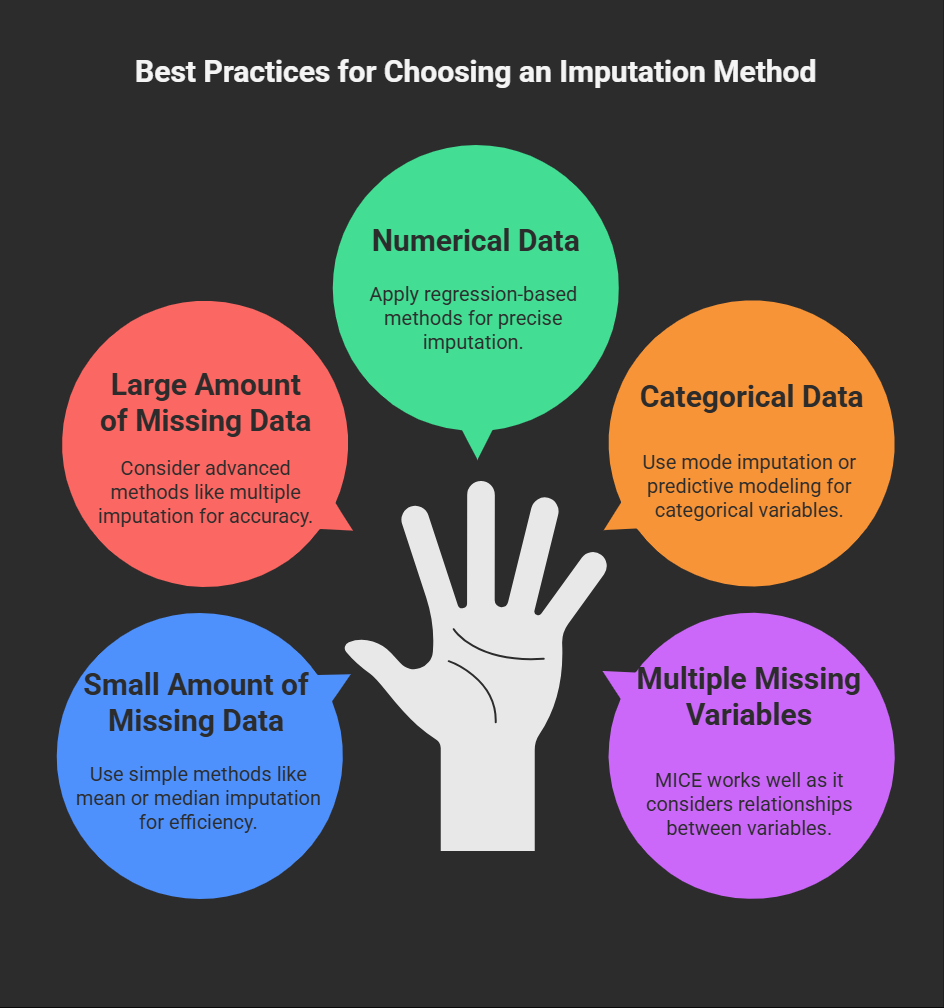
• Small Amount of Missing Data: For small amounts of missing data (less than 5%), simple methods like mean, median, or mode imputation often suffice.
• Large Amount of Missing Data: For larger amounts of missing data, advanced methods like KNN or MICE provide better estimates.
• Numerical Data: For numerical data, mean, median, or KNN imputation are commonly used.
• Categorical Data: For categorical variables, mode imputation or KNN imputation works well.
• Multiple Missing Variables: If you have many features with missing values, MICE is a robust choice as it accounts for interdependencies between variables.

Conclusion

Data imputation is a crucial step in the data preprocessing pipeline, ensuring that missing data doesn’t compromise the accuracy of machine learning models. While simple techniques like mean, median, and mode input a machine-learningtion are easy to implement, advanced methods like KNN and MICE offer more robust solutions by considering relationships between variables. Understanding the type of missing data and the context of your dataset will help you select the most appropriate imputation technique for your machine learning project.